SDDP.jl - A Flexible SDDP Library
Unless you can come up with a catchy name
- JAST.jl - Just Another SDDP Toolbox
- JEMSO.jl - JuMP Extension for Multi-stage Stochastic Optimisation
- Kokako.jl - a NZ bird
- Mohua.jl - Multistage Optimisation H?? Uncertainty A?? another NZ bird
- Moa.jl - Multistage Optimisation Application yet another NZ bird
Oscar Dowson, P.h.D. Candidate, The University of Auckland
Moa.jl
Q: Why another SDDP toolbox?
One year ago (ish) there weren't any! Now there are at least four!
- FAST (Finally An SDDP Toolbox) Released on Github a year ago although around previously
- StochDynamicProgramming.jl
- StructDualDynProg.jl
SDDP.jlMoa.jl
A: I'm a simple minded Engineer not a Mathematician
I think in terms of real variables (flow in = flow out), rather than linear algebra ($x_t = x_{t-1}$).
What this isn't
- It isn't able to switch between SDP and SDDP
- It isn't a $x, u, w$ matrix approach
Warning
I may play a little fast and loose with "proper" math notation and definitions...
What are we talking about...
- Multistage stochastic linear program in discrete time
- RHS uncertainty (scenarios)
- Markov uncertainty (see Philpott and de Matos)
- Risk Neutral (for now)
What are we talking about
A stage has six things

- An incoming state $x_{t-1}$
- An outgoing state $x_t$
- Uncertainty that is realised at the beginning of the state $\omega_t$
- An action that is taken $u_t$
- Some dynamics $x_t = f_t(x_{t-1}, u_t, \omega_t)$
- A reward that is earned $c_t(x_{t-1}, x_t, u_t)$
$SP_t$ is a user defined JuMP model.
Where this might differ
- If I record 6 different states (initial, + five more), there are five stages, not six;
- Wait-and-See in a stage. You take an action today after realising the uncertainty;
- Each stage is set-up as a linear programme.
We call the linear programme that defines a stage a subproblem.
# To get started we need to clone SDDP.jl
# Pkg.clone("https://github.com/odow/SDDP.jl")

# load some packages
using SDDP, JuMP, Clp
The stock example from StochDynamicProgramming.jl
Links to StochDynamicPrograming.jl and SDDP.jl versions.
- Sense
- Minimising
- Stages
- 5 stages ($t = 1,2,3,4,5$)
- States
- 1 State $x_t \in [0, 1]$ (initial state $x_0 = 0.5$)
- Controls
- 1 control $u_t \in [0, 0.5]$
- Noises
- 10 stagewise independent noises: $\omega_t \in [0, 0.0333..., 0.0666..., ..., 0.3]$
- Dynamics
- linear dynamics $x_t == x_{t-1} + u_t - \omega_t $
- Stage Objective
- linear objective $(\sin(3t) - 1) \cdot u_t$
Syntax for creating a new SDDPModel
We define 1. and 2. in the constructor using keyword arguments.
m = SDDPModel(
                  sense = :Min,          # :Max or :Min?
                 stages = 5,             # Number of stages
                 solver = ClpSolver(),   # AbstractMathProgSolver
           risk_measure = Expectation(), # plain old expectation
        objective_bound = -2             # Valid lower bound (since we're minimising)
                                        ) do sp, t
                                        # these can be called anything. i.e.
                                        # ) do subproblem_jump_model, stage_index
                                        # the first is a new JuMP Model for the subproblem, the second is an
                                        # index from 1,2,...,5

    # ... subproblem definition goes here ...

end
Defining the subproblem
We still need to define the last five things:
3. States
4. Controls
5. Noises
6. Dynamics
7. Objective
We're going to use both sp and t from above.
3. Defining a state
A stage has an incoming, and an outgoing state variable. Behind the scenes we'll take care of matching them up between stages.
To define a new state variable use the @state macro.
@state(sp, lb <= outgoing <= ub, incoming == initial value)
First argument is the subproblem variable from the constructor, second argument is the outgoing variable (any feasible JuMP variable definition), third argument is the incoming variable (symbol == initial value).
From above, we have one state $x_t\in[0,1],\quad x_0 = 0.5$
@state(sp, 0 <= x <= 1, x0 == 0.5)
The x0 is the incoming variable in each stage. It will only be forced to 0.5 in the first stage. The syntax is just for convinence.
We could also create three state variables $x^i_t \in [0, \infty),\quad x^i_0 = i, \quad i=\{1,2,3\}\quad t=\{1,2,\dots,T\}$
@state(sp, x[i=1:3] >= 0, x0==i)
or do fancier things like
RESERVOIRS = [:taupo, :benmore]
INITIAL_STORAGE = Dict(:taupo => 1, :benmore => 2)

@state(sp, x[r=RESERVOIRS] >= 0, x0==INITIAL_STORAGE[r])
Updating our model with the new state
m = SDDPModel(
                  sense = :Min,
                 stages = 5,
                 solver = ClpSolver(),
           risk_measure = Expectation(),
        objective_bound = -2
                                        ) do sp, t

    @state(sp, 0 <= x <= 1, x0 == 0.5)

    # ... subproblem definition goes here ...

end
4. Defining a control
Controls are just JuMP variables. Nothing special.
From above $u_t \in [0, 0.5]$
@variable(sp, 0 <= control <= 0.5)
Updating our model with the new control
m = SDDPModel(
                  sense = :Min,
                 stages = 5,
                 solver = ClpSolver(),
           risk_measure = Expectation(),
        objective_bound = -2
                                        ) do sp, t

    # the state
    @state(sp, 0 <= x <= 1, x0 == 0.5)

    # the control
    @variable(sp, 0 <= u <= 0.5)

    # ... subproblem definition goes here ...

end
5. Defining a Noise
Still a little messy. Not overly happy with it...
A noise has three things:
- A constraint
- A set of RHS values
- A probability distribution
Julia code is
@scenario(sp, name = RHS Values, constraint)

setscenarioprobability!(sp, probability distribution)
From above we have
5 - Noises
- 10 stagewise independent noises: $\omega_t \in [0, 0.0333..., 0.0666..., ..., 0.3]$
6 - Dynamics
- linear dynamics $x_t == x_{t-1} + u_t - \omega_t $
@scenario(sp, omega = linspace(0, 0.3, 10), x == x0 + u - omega)

# set uniform probability (but its the default so you don't have to
setscenarioprobability!(sp, fill(0.1, 10))
Updating out model with the new noise
m = SDDPModel(
                  sense = :Min,
                 stages = 5,
                 solver = ClpSolver(),
           risk_measure = Expectation(),
        objective_bound = -2
                                        ) do sp, t

    # the state
    @state(sp, 0 <= x <= 1, x0 == 0.5)

    # the control
    @variable(sp, 0 <= u <= 0.5)

    # the noise (and dynamics)
    @scenario(sp, omega = linspace(0, 0.3, 10), x == x0 + u - omega)

    # ... subproblem definition goes here ...

end
7. Defining the Stage Objective
We only care about defining the stage objective. The future costs get handled automatically.
stageobjective!(sp, AffExpr of Objective)
We can use the index t to change coefficients between subproblems so our objective is
stageobjective!(sp, (sin(3 * t) - 1) * u)
m = SDDPModel(
                  sense = :Min,
                 stages = 5,
                 solver = ClpSolver(),
           risk_measure = Expectation(),
        objective_bound = -2
                                        ) do sp, t

    # the state
    @state(sp, 0 <= x <= 1, x0 == 0.5)

    # the control
    @variable(sp, 0 <= u <= 0.5)

    # the noise (and dynamics)
    @scenario(sp, omega = linspace(0, 0.3, 10), x == x0 + u - omega)

    # the objective
    stageobjective!(sp, (sin(3 * t) - 1) * u)

end
println(typeof(m))
Compare the Julia code
m = SDDPModel(
                  sense = :Min,
                 stages = 5,
                 solver = ClpSolver(),
           risk_measure = Expectation(),
        objective_bound = -2
                                        ) do sp, t
    @state(sp,    0 <= x <= 1, x0 == 0.5)
    @variable(sp, 0 <= u <= 0.5)
    @scenario(sp, omega = linspace(0, 0.3, 10), x == x0 + u - omega)
    stageobjective!(sp, (sin(3t) - 1)*u )
end
to the mathematical subproblem
$ \begin{array}{r l} \min\limits_{u_t} & (sin(3t) - 1)u_t + \theta_{t+1}\\ s.t. & x_t = x_{t-1} + u_t - \omega_t \\ & x_t \in [0, 1] \\ & u_t \in [0, 0.5] \\ & x_0 = 0.5 \end{array} $
Solve options
For a full list run julia>? SDDP.solve
status = solve(m,
    max_iterations = 10,
    time_limit     = 600,
    simulation     = MonteCarloSimulation(
                        frequency = 5,
                        min       = 10,
                        step      = 10,
                        max       = 100,
                        terminate = false
                    )
)
srand(1111)
status = solve(m,
    max_iterations = 20,
    time_limit     = 600,
    simulation     = MonteCarloSimulation(
                        frequency = 5,
                        min       = 10,
                        step      = 10,
                        max       = 100,
                        termination = false
                    ),
    # print_level=0
)

# Check bound is correct
println("Final bound is $(SDDP.getbound(m)) (Expected -1.471).")
-------------------------------------------------------------------------------
                      SDDP Solver. © Oscar Dowson, 2017.
-------------------------------------------------------------------------------
    Solver:
        Serial solver
    Model:
        Stages:         5
        States:         1
        Subproblems:    5
        Value Function: Default
-------------------------------------------------------------------------------
              Objective              |  Cut  Passes    Simulations   Total
      Expected        Bound   % Gap  |   #     Time     #    Time    Time
-------------------------------------------------------------------------------
-1.591 -1.471 | 1 0.0 0 0.0 0.0
-1.365 -1.471 | 2 0.0 0 0.0 0.0
-1.518 -1.471 | 3 0.0 0 0.0 0.0
-1.624 -1.471 | 4 0.0 0 0.0 0.0
-1.569 -1.479 -1.471 -6.7 | 5 0.0 20 0.0 0.1
-1.537 -1.471 | 6 0.0 20 0.0 0.1
-1.387 -1.471 | 7 0.1 20 0.0 0.1
-1.403 -1.471 | 8 0.1 20 0.0 0.1
-1.567 -1.471 | 9 0.1 20 0.0 0.1
-1.491 -1.424 -1.471 -1.4 | 10 0.1 120 0.1 0.2
-1.347 -1.471 | 11 0.1 120 0.1 0.2
-1.456 -1.471 | 12 0.1 120 0.1 0.2
-1.525 -1.471 | 13 0.1 120 0.1 0.2
-1.801 -1.471 | 14 0.1 120 0.1 0.2
-1.524 -1.453 -1.471 -3.6 | 15 0.1 220 0.2 0.3
-1.746 -1.471 | 16 0.1 220 0.2 0.3
-1.276 -1.471 | 17 0.1 220 0.2 0.3
-1.285 -1.471 | 18 0.1 220 0.2 0.3
-1.236 -1.471 | 19 0.1 220 0.2 0.3
-1.505 -1.435 -1.471 -2.3 | 20 0.2 320 0.2 0.4
-------------------------------------------------------------------------------
Statistics:
Iterations: 20
Termination Status: max_iterations
-------------------------------------------------------------------------------
Final bound is -1.4710749176074305 (Expected -1.471).simulation = simulate(m, 1000, [:x, :u])
println("Mean of simulation objectives is $(mean(r[:objective] for r in simulation))")
@visualise(simulation, i, t, begin
    simulation[i][:x][t], (title="State")
    simulation[i][:u][t], (title="Control")
    simulation[i][:scenario][t], (title="Scenario")
    simulation[i][:stageobjective][t], (title="Objective", cumulative=true)
end)
Average Value at Risk
risk_measure = NestedAVaR(lambda = 0.5, beta = 0.5)
A risk measure that is a convex combination of Expectation and Average Value @ Risk (also called Conditional Value @ Risk).
lambda * E[x] + (1 - lambda) * AV@R(1-beta)[x]
Keyword Arguments
lambda
Convex weight on the expectation ((1-lambda) weight is put on the AV@R component.
Inreasing values of lambda are less risk averse (more weight on expecattion)
betaThe quantile at which to calculate the Average Value @ Risk. Increasing values of
betaare less risk averse. Ifbeta=0, then the AV@R component is the worst case risk measure.
m_risk = SDDPModel(
                  sense = :Min,
                 stages = 5,
                 solver = ClpSolver(),
           # risk_measure = Expectation(),
           risk_measure = NestedAVaR(lambda=0.5, beta=0.5),
        objective_bound = -2
                                        ) do sp, t

    # the state
    @state(sp, 0 <= x <= 1, x0 == 0.5)

    # the control
    @variable(sp, 0 <= u <= 0.5)

    # the noise (and dynamics)
    @scenario(sp, omega = linspace(0, 0.3, 10), x == x0 + u - omega)

    # the objective
    stageobjective!(sp, (sin(3 * t) - 1) * u)

end
println(typeof(m_risk))
srand(1111)
status = solve(m_risk,
    max_iterations = 20,
    time_limit     = 600,
    simulation     = MonteCarloSimulation(
                        frequency = 5,
                        min       = 10,
                        step      = 10,
                        max       = 100,
                        termination = false
                    ),
    print_level=0
)

# Check bound is correct
println("Final bound is $(SDDP.getbound(m_risk)) (Expectation bound was -1.471).")
-------------------------------------------------------------------------------
                      SDDP Solver. © Oscar Dowson, 2017.
-------------------------------------------------------------------------------
    Solver:
        Serial solver
    Model:
        Stages:         5
        States:         1
        Subproblems:    5
        Value Function: Default
-------------------------------------------------------------------------------
              Objective              |  Cut  Passes    Simulations   Total
      Expected        Bound   % Gap  |   #     Time     #    Time    Time
-------------------------------------------------------------------------------
       -1.359         -1.536         |     1    0.1      0    0.0    0.1
       -0.943         -1.419         |     2    0.2      0    0.0    0.2
       -1.512         -1.379         |     3    0.2      0    0.0    0.2
       -1.596         -1.365         |     4    0.2      0    0.0    0.2
  -1.555    -1.456    -1.363  -14.1  |     5    0.2     10    0.0    0.2
       -1.564         -1.362         |     6    0.2     10    0.0    0.2
       -1.533         -1.357         |     7    0.2     10    0.0    0.2
       -1.525         -1.354         |     8    0.2     10    0.0    0.2
       -1.689         -1.353         |     9    0.2     10    0.0    0.2
  -1.549    -1.436    -1.351  -14.6  |    10    0.2     20    0.0    0.2
       -1.603         -1.351         |    11    0.2     20    0.0    0.2
       -1.622         -1.350         |    12    0.2     20    0.0    0.2
       -1.482         -1.349         |    13    0.2     20    0.0    0.2
       -1.327         -1.349         |    14    0.2     20    0.0    0.2
  -1.571    -1.381    -1.348  -16.5  |    15    0.2     30    0.0    0.2
       -1.400         -1.347         |    16    0.2     30    0.0    0.2
       -1.400         -1.347         |    17    0.2     30    0.0    0.3
       -1.611         -1.347         |    18    0.2     30    0.0    0.3
       -1.415         -1.347         |    19    0.2     30    0.0    0.3
  -1.480    -1.382    -1.346   -9.9  |    20    0.2     60    0.0    0.3
-------------------------------------------------------------------------------
    Statistics:
        Iterations:         20
        Termination Status: max_iterations
-------------------------------------------------------------------------------
Final bound is -1.3463746517409778 (Expectation bound was -1.471).
De Matos (Level One) Cut Selection
m_risk = SDDPModel(
                  sense = :Min,
                 stages = 5,
                 solver = ClpSolver(),
           risk_measure = Expectation(),
        objective_bound = -2,
        cut_oracle      = DematosCutOracle()
                                        ) do sp, t
m_dematos = SDDPModel(
                  sense = :Min,
                 stages = 5,
                 solver = ClpSolver(),
           risk_measure = Expectation(),
        objective_bound = -2,
        cut_oracle      = DematosCutOracle()
                                        ) do sp, t

    # the state
    @state(sp, 0 <= x <= 1, x0 == 0.5)

    # the control
    @variable(sp, 0 <= u <= 0.5)

    # the noise (and dynamics)
    @scenario(sp, omega = linspace(0, 0.3, 10), x == x0 + u - omega)

    # the objective
    stageobjective!(sp, (sin(3 * t) - 1) * u)

end
println(typeof(m_dematos))
srand(1111)
status = solve(m_dematos,
    max_iterations = 20,
    time_limit     = 600,
    cut_selection_frequency = 5,
    simulation     = MonteCarloSimulation(
                        frequency = 5,
                        min       = 10,
                        step      = 10,
                        max       = 100,
                        termination = false
                    ),
    print_level=0
)

# Check bound is correct
println("\nFinal bound is $(SDDP.getbound(m_dematos)) (Expectation bound was -1.471).")

c = SDDP.valueoracle(SDDP.getsubproblem(m_dematos, 1, 1)).cutmanager

println("\nPercentage of discovered cuts kept in first stage $(100 * length(SDDP.validcuts(c)) / length(c.cuts))%")
-------------------------------------------------------------------------------
SDDP Solver. © Oscar Dowson, 2017.
-------------------------------------------------------------------------------
Solver:
Serial solver
Model:
Stages: 5
States: 1
Subproblems: 5
Value Function: Default
-------------------------------------------------------------------------------
Objective | Cut Passes Simulations Total
Expected Bound % Gap | # Time # Time Time
-------------------------------------------------------------------------------
-1.359 -1.743 | 1 0.1 0 0.0 0.1
-0.943 -1.594 | 2 0.1 0 0.0 0.1
-1.518 -1.530 | 3 0.1 0 0.0 0.1
-1.557 -1.502 | 4 0.1 0 0.0 0.2
-1.492 -1.443 -1.485 -0.5 | 5 0.2 100 0.0 0.3
-1.462 -1.483 | 6 0.2 100 0.0 0.3
-1.753 -1.478 | 7 0.2 100 0.0 0.3
-1.562 -1.476 | 8 0.2 100 0.0 0.3
-1.438 -1.475 | 9 0.2 100 0.0 0.3
-1.515 -1.438 -1.474 -2.8 | 10 0.2 200 0.1 0.4
-1.620 -1.474 | 11 0.2 200 0.1 0.4
-1.653 -1.473 | 12 0.2 200 0.1 0.4
-1.445 -1.473 | 13 0.2 200 0.1 0.4
-1.629 -1.473 | 14 0.2 200 0.1 0.4
-1.491 -1.421 -1.473 -1.3 | 15 0.2 300 0.2 0.5
-1.080 -1.473 | 16 0.2 300 0.2 0.5
-1.613 -1.472 | 17 0.2 300 0.2 0.5
-1.684 -1.472 | 18 0.2 300 0.2 0.5
-0.980 -1.472 | 19 0.2 300 0.2 0.5
-1.505 -1.431 -1.472 -2.2 | 20 0.2 400 0.2 0.5
-------------------------------------------------------------------------------
Statistics:
Iterations: 20
Termination Status: max_iterations
-------------------------------------------------------------------------------
Final bound is -1.4720242628387088 (Expectation bound was -1.471).

Percentage of discovered cuts kept in first stage 25.0%Asyncronous Solver
We parallelise by farming out a new instance of the SDDPModel to all slave processors.
Slaves perform iterations independently, and asyncronously share cuts between themselves.
solve(m,
    solve_type = Serial()
    # or
    solve_type = Asyncronous()
)
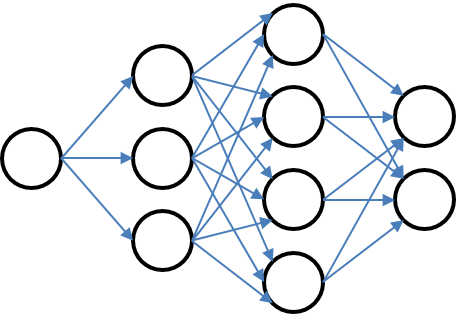
Markov Uncertainty
More like a feed-forward graph with discrete stages but arbitrary number of nodes and transitions

# Transition[last index, current_index] = probability
Transition = Array{Float64, 2}[
    [1.0],
    [0.5 0.5],
    [0.25 0.75; 0.75 0.25],
    [0.25 0.75; 0.75 0.25],
    [0.25 0.75; 0.75 0.25]
]
Transition = Array{Float64, 2}[
    [1.0]',
    [0.5 0.5],
    [0.25 0.75; 0.75 0.25],
    [0.25 0.75; 0.75 0.25],
    [0.25 0.75; 0.75 0.25]
]

m_markov = SDDPModel(
                  sense = :Min,
                 stages = 5,
                 solver = ClpSolver(),
        objective_bound = -10,
        # A vector of transition matrices. One for each stage
      markov_transition = Transition
                                        # markov_state will go from 1, 2, ..., S
                                        ) do sp, t, markov_state
    @state(sp, 0 <= x <= 1, x0 == 0.5)
    @variable(sp, 0 <= u <= 0.5)
    @scenario(sp, omega = linspace(0, 0.3, 10), x == x0 + u - omega)

    # the objective
    stageobjective!(sp, (sin(3 * t) - 0.75 * markov_state) * u)

end
println(typeof(m_markov))
status = solve(m_markov,
    max_iterations = 10
)

# Check bound is correct
println("Final bound is $(SDDP.getbound(m_markov)).")
Extensions
The code is extensible. It's possible to add new features. Risk measures, cut managers, etc.
SDDiP
@lkapelevich is currently writing a Lagrangian solver for SDDiP. It turns out to be a trivial extension and everything "just works".
Going Forward
- It needs documentation;
- It needs a bit of a refactor and a tidy;
- I need to understand the differences better between libraries.
Cut Managers
- Common "cut" type
- Common API
- Store cut
- Store state
- Get valid cuts
Risk Measures
- Common API.
modifyprobabilty!(measure::AbstractRiskMeasure, new_probabilities, old_probabilities, objectives, sense)
SDP
Take a look at DynamicProgramming.jl.
It's not well tested or documented, but it has a nice syntax. Links in with the Javascript visualisation.