An introduction to SDDP.jl

This tutorial was generated using Literate.jl. Download the source as a .jl file. Download the source as a .ipynb file.

SDDP.jl is a solver for multistage stochastic optimization problems. By multistage, we mean problems in which an agent makes a sequence of decisions over time. By stochastic, we mean that the agent is making decisions in the presence of uncertainty that is gradually revealed over the multiple stages.

This tutorial is in two parts. First, it is an introduction to the background notation and theory we need, and second, it solves a simple multistage stochastic programming problem.

What is a node?

A common feature of multistage stochastic optimization problems is that they model an agent controlling a system over time. To simplify things initially, we're going to start by describing what happens at an instant in time at which the agent makes a decision. Only after this will we extend our problem to multiple stages and the notion of time.

A node is a place at which the agent makes a decision.

States, controls, and random variables

The system that we are modeling can be described by three types of variables.

1. State variables track a property of the system over time.

   Each node has an associated incoming state variable (the value of the state at the start of the node), and an outgoing state variable (the value of the state at the end of the node).

   Examples of state variables include the volume of water in a reservoir, the number of units of inventory in a warehouse, or the spatial position of a moving vehicle.

   Because state variables track the system over time, each node must have the same set of state variables.

   We denote state variables by the letter $x$ for the incoming state variable and $x^\prime$ for the outgoing state variable.

2. Control variables are actions taken (implicitly or explicitly) by the agent within a node which modify the state variables.

   Examples of control variables include releases of water from the reservoir, sales or purchasing decisions, and acceleration or braking of the vehicle.

   Control variables are local to a node $i$, and they can differ between nodes. For example, some control variables may be available within certain nodes.

   We denote control variables by the letter $u$.

3. Random variables are finite, discrete, exogenous random variables that the agent observes at the start of a node, before the control variables are decided.

   Examples of random variables include rainfall inflow into a reservoir, probabilistic perishing of inventory, and steering errors in a vehicle.

   Random variables are local to a node $i$, and they can differ between nodes. For example, some nodes may have random variables, and some nodes may not.

   We denote random variables by the Greek letter $\omega$ and the sample space from which they are drawn by $\Omega_i$. The probability of sampling $\omega$ is denoted $p_{\omega}$ for simplicity.

   Importantly, the random variable associated with node $i$ is independent of the random variables in all other nodes.

Dynamics

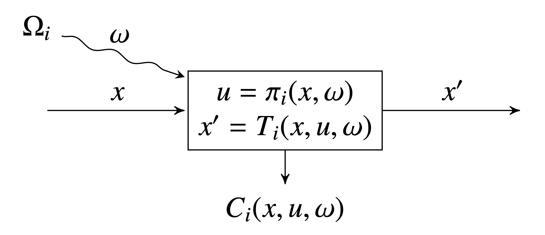
In a node $i$, the three variables are related by a transition function, which maps the incoming state, the controls, and the random variables to the outgoing state as follows: $x^\prime = T_i(x, u, \omega)$.

As a result of entering a node $i$ with the incoming state $x$, observing random variable $\omega$, and choosing control $u$, the agent incurs a cost $C_i(x, u, \omega)$. (If the agent is a maximizer, this can be a profit, or a negative cost.) We call $C_i$ the stage objective.

To choose their control variables in node $i$, the agent uses a decision rule $u = \pi_i(x, \omega)$, which is a function that maps the incoming state variable and observation of the random variable to a control $u$. This control must satisfy some feasibility requirements $u \in U_i(x, \omega)$.

Here is a schematic which we can use to visualize a single node:

Policy graphs

Now that we have a node, we need to connect multiple nodes together to form a multistage stochastic program. We call the graph created by connecting nodes together a policy graph.

The simplest type of policy graph is a linear policy graph. Here's a linear policy graph with three nodes:

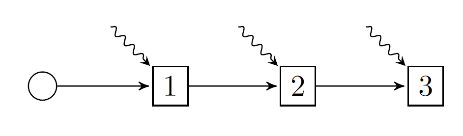
Here we have dropped the notations inside each node and replaced them by a label (1, 2, and 3) to represent nodes i=1, i=2, and i=3.

In addition to nodes 1, 2, and 3, there is also a root node (the circle), and three arcs. Each arc has an origin node and a destination node, like 1 => 2, and a corresponding probability of transitioning from the origin to the destination. Unless specified, we assume that the arc probabilities are uniform over the number of outgoing arcs. Thus, in this picture the arc probabilities are all 1.0.

State variables flow long the arcs of the graph. Thus, the outgoing state variable $x^\prime$ from node 1 becomes the incoming state variable $x$ to node 2, and so on.

We denote the set of nodes by $\mathcal{N}$, the root node by $R$, and the probability of transitioning from node $i$ to node $j$ by $p_{ij}$. (If no arc exists, then $p_{ij} = 0$.) We define the set of successors of node $i$ as $i^+ = \{j \in \mathcal{N} | p_{ij} > 0\}$.

Each node in the graph corresponds to a place at which the agent makes a decision, and we call moments in time at which the agent makes a decision stages. By convention, we try to draw policy graphs from left-to-right, with the stages as columns. There can be more than one node in a stage! Here's an example of a structure we call Markovian policy graphs:

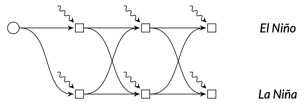
Here each column represents a moment in time, the squiggly lines represent stochastic rainfall, and the rows represent the world in two discrete states: El Niño and La Niña. In the El Niño states, the distribution of the rainfall random variable is different to the distribution of the rainfall random variable in the La Niña states, and there is some switching probability between the two states that can be modelled by a Markov chain.

Moreover, policy graphs can have cycles! This allows them to model infinite horizon problems. Here's another example, taken from the paper Dowson (2020):

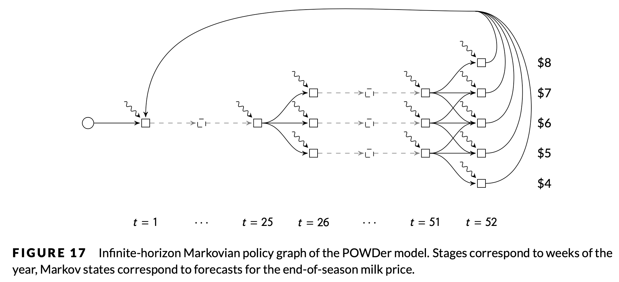
The columns represent time, and the rows represent different states of the world. In this case, the rows represent different prices that milk can be sold for at the end of each year. The squiggly lines denote a multivariate random variable that models the weekly amount of rainfall that occurs.

More notation

Recall that each node $i$ has a decision rule $u = \pi_i(x, \omega)$, which is a function that maps the incoming state variable and observation of the random variable to a control $u$.

The set of decision rules, with one element for each node in the policy graph, is called a policy.

The goal of the agent is to find a policy that minimizes the expected cost of starting at the root node with some initial condition $x_R$, and proceeding from node to node along the probabilistic arcs until they reach a node with no outgoing arcs (or it reaches an implicit "zero" node).

\[\min_{\pi} \mathbb{E}_{i \in R^+, \omega \in \Omega_i}[V_i^\pi(x_R, \omega)],\]

where

\[V_i^\pi(x, \omega) = C_i(x, u, \omega) + \mathbb{E}_{j \in i^+, \varphi \in \Omega_j}[V_j(x^\prime, \varphi)],\]

where $u = \pi_i(x, \omega) \in U_i(x, \omega)$, and $x^\prime = T_i(x, u, \omega)$.

The expectations are a bit complicated, but they are equivalent to:

\[\mathbb{E}_{j \in i^+, \varphi \in \Omega_j}[V_j(x^\prime, \varphi)] = \sum\limits_{j \in i^+} p_{ij} \sum\limits_{\varphi \in \Omega_j} p_{\varphi}V_j(x^\prime, \varphi).\]

An optimal policy is the set of decision rules that the agent can use to make decisions and achieve the smallest expected cost.

Assumptions

The space of problems you can model with this framework is very large. Too large, in fact, for us to form tractable solution algorithms for! Stochastic dual dynamic programming requires the following assumptions in order to work:

Assumption 1: finite nodes

There is a finite number of nodes in $\mathcal{N}$.

Assumption 2: finite random variables

The sample space $\Omega_i$ is finite and discrete for each node $i\in\mathcal{N}$.

Assumption 3: convex problems

Given fixed $\omega$, $C_i(x, u, \omega)$ is a convex function, $T_i(x, u, \omega)$ is linear, and $U_i(x, u, \omega)$ is a non-empty, bounded convex set with respect to $x$ and $u$.

Assumption 4: no infinite loops

For all loops in the policy graph, the product of the arc transition probabilities around the loop is strictly less than 1.

Assumption 5: relatively complete recourse

This is a technical but important assumption. See Relatively complete recourse for more details.

Dynamic programming and subproblems

Now that we have formulated our problem, we need some ways of computing optimal decision rules. One way is to just use a heuristic like "choose a control randomly from the set of feasible controls." However, such a policy is unlikely to be optimal.

A better way of obtaining an optimal policy is to use Bellman's principle of optimality, a.k.a Dynamic Programming, and define a recursive subproblem as follows:

\[\begin{aligned} V_i(x, \omega) = \min\limits_{\bar{x}, x^\prime, u} \;\; & C_i(\bar{x}, u, \omega) + \mathbb{E}_{j \in i^+, \varphi \in \Omega_j}[V_j(x^\prime, \varphi)]\\ & x^\prime = T_i(\bar{x}, u, \omega) \\ & u \in U_i(\bar{x}, \omega) \\ & \bar{x} = x. \end{aligned}\]

Our decision rule, $\pi_i(x, \omega)$, solves this optimization problem and returns a $u^*$ corresponding to an optimal solution.

These subproblems are very difficult to solve exactly, because they involve recursive optimization problems with lots of nested expectations.

Therefore, instead of solving them exactly, SDDP.jl works by iteratively approximating the expectation term of each subproblem, which is also called the cost-to-go term. For now, you don't need to understand the details, other than that there is a nasty cost-to-go term that we deal with behind-the-scenes.

The subproblem view of a multistage stochastic program is also important, because it provides a convenient way of communicating the different parts of the broader problem, and it is how we will communicate the problem to SDDP.jl. All we need to do is drop the cost-to-go term and fishing constraint, and define a new subproblem SP as:

\[\begin{aligned} \texttt{SP}_i(x, \omega) : \min\limits_{\bar{x}, x^\prime, u} \;\; & C_i(\bar{x}, u, \omega) \\ & x^\prime = T_i(\bar{x}, u, \omega) \\ & u \in U_i(\bar{x}, \omega). \end{aligned}\]

We've retained the transition function and uncertainty set because they help to motivate the different components of the subproblem. However, in general, the subproblem can be more general. A better (less restrictive) representation might be:

\[\begin{aligned} \texttt{SP}_i(x, \omega) : \min\limits_{\bar{x}, x^\prime, u} \;\; & C_i(\bar{x}, x^\prime, u, \omega) \\ & (\bar{x}, x^\prime, u) \in \mathcal{X}_i(\omega). \end{aligned}\]

Note that the outgoing state variable can appear in the objective, and we can add constraints involving the incoming and outgoing state variables. It should be obvious how to map between the two representations.

Example: hydro-thermal scheduling

Hydrothermal scheduling is the most common application of stochastic dual dynamic programming. To illustrate some of the basic functionality of SDDP.jl, we implement a very simple model of the hydrothermal scheduling problem.

Problem statement

We consider the problem of scheduling electrical generation over three weeks in order to meet a known demand of 150 MWh in each week.

There are two generators: a thermal generator, and a hydro generator. In each week, the agent needs to decide how much energy to generate from thermal, and how much energy to generate from hydro.

The thermal generator has a short-run marginal cost of $50/MWh in the first stage, $100/MWh in the second stage, and $150/MWh in the third stage.

The hydro generator has a short-run marginal cost of $0/MWh.

The hydro generator draws water from a reservoir which has a maximum capacity of 200 MWh. (Although water is usually measured in m³, we measure it in the energy-equivalent MWh to simplify things. In practice, there is a conversion function between m³ flowing throw the turbine and MWh.) At the start of the first time period, the reservoir is full.

In addition to the ability to generate electricity by passing water through the hydroelectric turbine, the hydro generator can also spill water down a spillway (bypassing the turbine) in order to prevent the water from over-topping the dam. We assume that there is no cost of spillage.

In addition to water leaving the reservoir, water that flows into the reservoir through rainfall or rivers are referred to as inflows. These inflows are uncertain, and are the cause of the main trade-off in hydro-thermal scheduling: the desire to use water now to generate cheap electricity, against the risk that future inflows will be low, leading to blackouts or expensive thermal generation.

For our simple model, we assume that the inflows can be modelled by a discrete distribution with the three outcomes given in the following table:

The value of the noise (the random variable) is observed by the agent at the start of each stage. This makes the problem a wait-and-see or hazard-decision formulation.

The goal of the agent is to minimize the expected cost of generation over the three weeks.

Formulating the problem

Before going further, we need to load SDDP.jl:

using SDDP

Graph structure

First, we need to identify the structure of the policy graph. From the problem statement, we want to model the problem over three weeks in weekly stages. Therefore, the policy graph is a linear graph with three stages:

graph = SDDP.LinearGraph(3)

Root
 0
Nodes
 1
 2
 3
Arcs
 0 => 1 w.p. 1.0
 1 => 2 w.p. 1.0
 2 => 3 w.p. 1.0

Building the subproblem

Next, we need to construct the associated subproblem for each node in graph. To do so, we need to provide SDDP.jl a function which takes two arguments. The first is subproblem::Model, which is an empty JuMP model. The second is node, which is the name of each node in the policy graph. If the graph is linear, SDDP defaults to naming the nodes using the integers in 1:T. Here's an example that we are going to flesh out over the next few paragraphs:

function subproblem_builder(subproblem::Model, node::Int)
    # ... stuff to go here ...
    return subproblem
end

subproblem_builder (generic function with 1 method)

State variables

The first part of the subproblem we need to identify are the state variables. Since we only have one reservoir, there is only one state variable, volume, the volume of water in the reservoir [MWh].

The volume had bounds of [0, 200], and the reservoir was full at the start of time, so $x_R = 200$.

We add state variables to our subproblem using JuMP's @variable macro. However, in addition to the usual syntax, we also pass SDDP.State, and we need to provide the initial value ($x_R$) using the initial_value keyword.

function subproblem_builder(subproblem::Model, node::Int)
    # State variables
    @variable(subproblem, 0 <= volume <= 200, SDDP.State, initial_value = 200)
    return subproblem
end

subproblem_builder (generic function with 1 method)

The syntax for adding a state variable is a little obtuse, because volume is not single JuMP variable. Instead, volume is a struct with two fields, .in and .out, corresponding to the incoming and outgoing state variables respectively.

Control variables

The next part of the subproblem we need to identify are the control variables. The control variables for our problem are:

• thermal_generation: the quantity of energy generated from thermal [MWh/week]
• hydro_generation: the quantity of energy generated from hydro [MWh/week]
• hydro_spill: the volume of water spilled from the reservoir in each week [MWh/week]

Each of these variables is non-negative.

We add control variables to our subproblem as normal JuMP variables, using @variable or @variables:

function subproblem_builder(subproblem::Model, node::Int)
    # State variables
    @variable(subproblem, 0 <= volume <= 200, SDDP.State, initial_value = 200)
    # Control variables
    @variables(subproblem, begin
        thermal_generation >= 0
        hydro_generation >= 0
        hydro_spill >= 0
    end)
    return subproblem
end

subproblem_builder (generic function with 1 method)

Random variables

The next step is to identify any random variables. In our example, we had

• inflow: the quantity of water that flows into the reservoir each week [MWh/week]

To add an uncertain variable to the model, we create a new JuMP variable inflow, and then call the function SDDP.parameterize. The SDDP.parameterize function takes three arguments: the subproblem, a vector of realizations, and a corresponding vector of probabilities.

function subproblem_builder(subproblem::Model, node::Int)
    # State variables
    @variable(subproblem, 0 <= volume <= 200, SDDP.State, initial_value = 200)
    # Control variables
    @variables(subproblem, begin
        thermal_generation >= 0
        hydro_generation >= 0
        hydro_spill >= 0
    end)
    # Random variables
    @variable(subproblem, inflow)
    Ω = [0.0, 50.0, 100.0]
    P = [1 / 3, 1 / 3, 1 / 3]
    SDDP.parameterize(subproblem, Ω, P) do ω
        return JuMP.fix(inflow, ω)
    end
    return subproblem
end

subproblem_builder (generic function with 1 method)

Note how we use the JuMP function JuMP.fix to set the value of the inflow variable to ω.

Transition function and constraints

Now that we've identified our variables, we can define the transition function and the constraints.

For our problem, the state variable is the volume of water in the reservoir. The volume of water decreases in response to water being used for hydro generation and spillage. So the transition function is: volume.out = volume.in - hydro_generation - hydro_spill + inflow. (Note how we use volume.in and volume.out to refer to the incoming and outgoing state variables.)

There is also a constraint that the total generation must sum to 150 MWh.

Both the transition function and any additional constraint are added using JuMP's @constraint and @constraints macro.

function subproblem_builder(subproblem::Model, node::Int)
    # State variables
    @variable(subproblem, 0 <= volume <= 200, SDDP.State, initial_value = 200)
    # Control variables
    @variables(subproblem, begin
        thermal_generation >= 0
        hydro_generation >= 0
        hydro_spill >= 0
    end)
    # Random variables
    @variable(subproblem, inflow)
    Ω = [0.0, 50.0, 100.0]
    P = [1 / 3, 1 / 3, 1 / 3]
    SDDP.parameterize(subproblem, Ω, P) do ω
        return JuMP.fix(inflow, ω)
    end
    # Transition function and constraints
    @constraints(
        subproblem,
        begin
            volume.out == volume.in - hydro_generation - hydro_spill + inflow
            demand_constraint, hydro_generation + thermal_generation == 150
        end
    )
    return subproblem
end

subproblem_builder (generic function with 1 method)

Objective function

Finally, we need to add an objective function using @stageobjective. The objective of the agent is to minimize the cost of thermal generation. This is complicated by a fuel cost that depends on the node.

One possibility is to use an if statement on node to define the correct objective:

function subproblem_builder(subproblem::Model, node::Int)
    # State variables
    @variable(subproblem, 0 <= volume <= 200, SDDP.State, initial_value = 200)
    # Control variables
    @variables(subproblem, begin
        thermal_generation >= 0
        hydro_generation >= 0
        hydro_spill >= 0
    end)
    # Random variables
    @variable(subproblem, inflow)
    Ω = [0.0, 50.0, 100.0]
    P = [1 / 3, 1 / 3, 1 / 3]
    SDDP.parameterize(subproblem, Ω, P) do ω
        return JuMP.fix(inflow, ω)
    end
    # Transition function and constraints
    @constraints(
        subproblem,
        begin
            volume.out == volume.in - hydro_generation - hydro_spill + inflow
            demand_constraint, hydro_generation + thermal_generation == 150
        end
    )
    # Stage-objective
    if node == 1
        @stageobjective(subproblem, 50 * thermal_generation)
    elseif node == 2
        @stageobjective(subproblem, 100 * thermal_generation)
    else
        @assert node == 3
        @stageobjective(subproblem, 150 * thermal_generation)
    end
    return subproblem
end

subproblem_builder (generic function with 1 method)

A second possibility is to use an array of fuel costs, and use node to index the correct value:

function subproblem_builder(subproblem::Model, node::Int)
    # State variables
    @variable(subproblem, 0 <= volume <= 200, SDDP.State, initial_value = 200)
    # Control variables
    @variables(subproblem, begin
        thermal_generation >= 0
        hydro_generation >= 0
        hydro_spill >= 0
    end)
    # Random variables
    @variable(subproblem, inflow)
    Ω = [0.0, 50.0, 100.0]
    P = [1 / 3, 1 / 3, 1 / 3]
    SDDP.parameterize(subproblem, Ω, P) do ω
        return JuMP.fix(inflow, ω)
    end
    # Transition function and constraints
    @constraints(
        subproblem,
        begin
            volume.out == volume.in - hydro_generation - hydro_spill + inflow
            demand_constraint, hydro_generation + thermal_generation == 150
        end
    )
    # Stage-objective
    fuel_cost = [50, 100, 150]
    @stageobjective(subproblem, fuel_cost[node] * thermal_generation)
    return subproblem
end

subproblem_builder (generic function with 1 method)

Constructing the model

Now that we've written our subproblem, we need to construct the full model. For that, we're going to need a linear solver. Let's choose HiGHS:

using HiGHS

Then, we can create a full model using SDDP.PolicyGraph, passing our subproblem_builder function as the first argument, and our graph as the second:

model = SDDP.PolicyGraph(
    subproblem_builder,
    graph;
    sense = :Min,
    lower_bound = 0.0,
    optimizer = HiGHS.Optimizer,
)

A policy graph with 3 nodes.
 Node indices: 1, 2, 3

• sense: the optimization sense. Must be :Min or :Max.
• lower_bound: you must supply a valid bound on the objective. For our problem, we know that we cannot incur a negative cost so $0 is a valid lower bound.
• optimizer: This is borrowed directly from JuMP's Model constructor: Model(HiGHS.Optimizer)

Because linear policy graphs are the most commonly used structure, we can use SDDP.LinearPolicyGraph instead of passing SDDP.LinearGraph(3) to SDDP.PolicyGraph.

model = SDDP.LinearPolicyGraph(
    subproblem_builder;
    stages = 3,
    sense = :Min,
    lower_bound = 0.0,
    optimizer = HiGHS.Optimizer,
)

A policy graph with 3 nodes.
 Node indices: 1, 2, 3

There is also the option is to use Julia's do syntax to avoid needing to define a subproblem_builder function separately:

model = SDDP.LinearPolicyGraph(
    stages = 3,
    sense = :Min,
    lower_bound = 0.0,
    optimizer = HiGHS.Optimizer,
) do subproblem, node
    # State variables
    @variable(subproblem, 0 <= volume <= 200, SDDP.State, initial_value = 200)
    # Control variables
    @variables(subproblem, begin
        thermal_generation >= 0
        hydro_generation >= 0
        hydro_spill >= 0
    end)
    # Random variables
    @variable(subproblem, inflow)
    Ω = [0.0, 50.0, 100.0]
    P = [1 / 3, 1 / 3, 1 / 3]
    SDDP.parameterize(subproblem, Ω, P) do ω
        return JuMP.fix(inflow, ω)
    end
    # Transition function and constraints
    @constraints(
        subproblem,
        begin
            volume.out == volume.in - hydro_generation - hydro_spill + inflow
            demand_constraint, hydro_generation + thermal_generation == 150
        end
    )
    # Stage-objective
    if node == 1
        @stageobjective(subproblem, 50 * thermal_generation)
    elseif node == 2
        @stageobjective(subproblem, 100 * thermal_generation)
    else
        @assert node == 3
        @stageobjective(subproblem, 150 * thermal_generation)
    end
end

A policy graph with 3 nodes.
 Node indices: 1, 2, 3

outer(inner::Function, x, y) = inner(x, y)

outer(1, 2) do x, y
    return x^2 + y^2
end

outer((x, y) -> x^2 + y^2, 1, 2)

Training a policy

Now we have a model, which is a description of the policy graph, we need to train a policy. Models can be trained using the SDDP.train function. It accepts a number of keyword arguments. iteration_limit terminates the training after the provided number of iterations.

SDDP.train(model; iteration_limit = 10)

-------------------------------------------------------------------
         SDDP.jl (c) Oscar Dowson and contributors, 2017-23
-------------------------------------------------------------------
problem
  nodes           : 3
  state variables : 1
  scenarios       : 2.70000e+01
  existing cuts   : false
options
  solver          : serial mode
  risk measure    : SDDP.Expectation()
  sampling scheme : SDDP.InSampleMonteCarlo
subproblem structure
  VariableRef                             : [7, 7]
  AffExpr in MOI.EqualTo{Float64}         : [2, 2]
  VariableRef in MOI.GreaterThan{Float64} : [5, 5]
  VariableRef in MOI.LessThan{Float64}    : [1, 2]
numerical stability report
  matrix range     [1e+00, 1e+00]
  objective range  [1e+00, 2e+02]
  bounds range     [2e+02, 2e+02]
  rhs range        [2e+02, 2e+02]
-------------------------------------------------------------------
 iteration    simulation      bound        time (s)     solves  pid
-------------------------------------------------------------------
         1   3.750000e+04  2.500000e+03  3.909111e-03        12   1
        10   1.750000e+04  8.333333e+03  1.426506e-02       120   1
-------------------------------------------------------------------
status         : iteration_limit
total time (s) : 1.426506e-02
total solves   : 120
best bound     :  8.333333e+03
simulation ci  :  1.362500e+04 ± 6.288333e+03
numeric issues : 0
-------------------------------------------------------------------

There's a lot going on in this printout! Let's break it down.

The first section, "problem," gives some problem statistics. In this example there are 3 nodes, 1 state variable, and 27 scenarios ($3^3$). We haven't solved this problem before so there are no existing cuts.

The "options" section lists some options we are using to solve the problem. For more information on the numerical stability report, read the Numerical stability report section.

The "subproblem structure" section also needs explaining. This looks at all of the nodes in the policy graph and reports the minimum and maximum number of variables and each constraint type in the corresponding subproblem. In this case each subproblem has 7 variables and various numbers of different constraint types. Note that the exact numbers may not correspond to the formulation as you wrote it, because SDDP.jl adds some extra variables for the cost-to-go function.

Then comes the iteration log, which is the main part of the printout. It has the following columns:

• iteration: the SDDP iteration
• simulation: the cost of the single forward pass simulation for that iteration. This value is stochastic and is not guaranteed to improve over time. However, it's useful to check that the units are reasonable, and that it is not deterministic if you intended for the problem to be stochastic, etc.
• bound: this is a lower bound (upper if maximizing) for the value of the optimal policy. This should be monotonically improving (increasing if minimizing, decreasing if maximizing).
• time (s): the total number of seconds spent solving so far
• solves: the total number of subproblem solves to date. This can be very large!
• pid: the ID of the processor used to solve that iteration. This should be 1 unless you are using parallel computation.

In addition, if the first character of a line is †, then SDDP.jl experienced numerical issues during the solve, but successfully recovered.

The printout finishes with some summary statistics:

• status: why did the solver stop?
• total time (s), best bound, and total solves are the values from the last iteration of the solve.
• simulation ci: a confidence interval that estimates the quality of the policy from the Simulation column.
• numeric issues: the number of iterations that experienced numerical issues.

Obtaining the decision rule

After training a policy, we can create a decision rule using SDDP.DecisionRule:

rule = SDDP.DecisionRule(model; node = 1)

A decision rule for node 1

Then, to evaluate the decision rule, we use SDDP.evaluate:

solution = SDDP.evaluate(
    rule;
    incoming_state = Dict(:volume => 150.0),
    noise = 50.0,
    controls_to_record = [:hydro_generation, :thermal_generation],
)

(stage_objective = 7500.0, outgoing_state = Dict(:volume => 200.0), controls = Dict(:thermal_generation => 150.0, :hydro_generation => -0.0))

Simulating the policy

Once you have a trained policy, you can also simulate it using SDDP.simulate. The return value from simulate is a vector with one element for each replication. Each element is itself a vector, with one element for each stage. Each element, corresponding to a particular stage in a particular replication, is a dictionary that records information from the simulation.

simulations = SDDP.simulate(
    # The trained model to simulate.
    model,
    # The number of replications.
    100,
    # A list of names to record the values of.
    [:volume, :thermal_generation, :hydro_generation, :hydro_spill],
)

replication = 1
stage = 2
simulations[replication][stage]

Dict{Symbol, Any} with 10 entries:
  :volume             => State{Float64}(200.0, 150.0)
  :hydro_spill        => 0.0
  :bellman_term       => 0.0
  :noise_term         => 100.0
  :node_index         => 2
  :stage_objective    => 0.0
  :objective_state    => nothing
  :thermal_generation => 0.0
  :hydro_generation   => 150.0
  :belief             => Dict(2=>1.0)

Ignore many of the entries for now; they will be relevant later.

One element of interest is :volume.

outgoing_volume = map(simulations[1]) do node
    return node[:volume].out
end

3-element Vector{Float64}:
 200.0
 150.0
   0.0

Another is :thermal_generation.

thermal_generation = map(simulations[1]) do node
    return node[:thermal_generation]
end

3-element Vector{Float64}:
 50.0
  0.0
  0.0

Obtaining bounds

Because the optimal policy is stochastic, one common approach to quantify the quality of the policy is to construct a confidence interval for the expected cost by summing the stage objectives along each simulation.

objectives = map(simulations) do simulation
    return sum(stage[:stage_objective] for stage in simulation)
end

μ, ci = SDDP.confidence_interval(objectives)
println("Confidence interval: ", μ, " ± ", ci)

Confidence interval: 9375.0 ± 973.482112954534

This confidence interval is an estimate for an upper bound of the policy's quality. We can calculate the lower bound using SDDP.calculate_bound.

println("Lower bound: ", SDDP.calculate_bound(model))

Lower bound: 8333.333333333332

Custom recorders

In addition to simulating the primal values of variables, we can also pass custom recorder functions. Each of these functions takes one argument, the JuMP subproblem corresponding to each node. This function gets called after we have solved each node as we traverse the policy graph in the simulation.

For example, the dual of the demand constraint (which we named demand_constraint) corresponds to the price we should charge for electricity, since it represents the cost of each additional unit of demand. To calculate this, we can go:

simulations = SDDP.simulate(
    model,
    1,  ## Perform a single simulation
    custom_recorders = Dict{Symbol,Function}(
        :price => (sp::JuMP.Model) -> JuMP.dual(sp[:demand_constraint]),
    ),
)

prices = map(simulations[1]) do node
    return node[:price]
end

3-element Vector{Float64}:
 50.0
 50.0
 -0.0

Extracting the marginal water values

Finally, we can use SDDP.ValueFunction and SDDP.evaluate to obtain and evaluate the value function at different points in the state-space.

First, we construct a value function from the first subproblem:

V = SDDP.ValueFunction(model; node = 1)

A value function for node 1

Then we can evaluate V at a point:

cost, price = SDDP.evaluate(V, Dict("volume" => 10))

(21499.999999999996, Dict(:volume => -99.99999999999999))

This returns the cost-to-go (cost), and the gradient of the cost-to-go function with respect to each state variable. Note that since we are minimizing, the price has a negative sign: each additional unit of water leads to a decrease in the expected long-run cost.